Enlighten Tutorial 2: enzyme with co-factor

As an example of an enzyme system with a (non-covalently bound) co-factor, we will use an NADP(H) containing reductase enzyme: isopiperitenone reductase. The starting point is PDB 5LDG, the structure of isopiperitenone reductase complexed with its substrate and NADP (see further this paper). We will need to supply parameters for the NADP co-factor.

NB: Whenever text is written in a box like this, it is a command that should be typed on a “command line”, either in a “terminal” or in the PyMOL control panel.

NB: Before running Enlighten2 through PyMOL, ensure that Docker is installed and running in the background.

Part 1: Preparing the model and co-factor parameters

We will use PyMOL to obtain the crystal structure we need directly from the protein databank. In the control panel type:

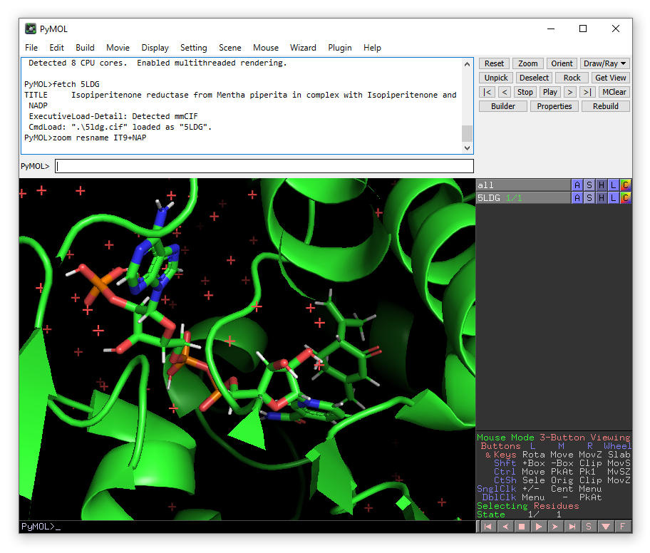
fetch 5LDG

A crystal structure will appear in the viewing window. You will also see an object called 5LDG appear in the right-hand viewing panel. There are buttons A,S,H etc. which contain drop down menus that allow you to make changes to how the object is viewed. You can zoom in on the isopiperitenone substrate and NADP(H) (which have residue names IT9 and NAP respectively):

zoom resname IT9+NAP

You will notice that in this PDB, hydrogen atoms are already present. This means that in principle, we can start using Enlighten directly on this object. But we will need to define parameters for the NADP co-factor. To do this, we will need two additional files:

• A ‘topology’ file that ‘translates’ atom names (from the PDB) into atom types, sets which ‘partial charges’ these atoms will have, and defines how they are bonded to each other. This file defines the molecule (co-factor), so that parameters can be assigned. For Amber/AmberTools, these files typically have the extensions .prep, .prepc, or .off
• A ‘parameter’ file with any parameters between the atom types in the co-factor that are not ‘known’ in the standard force field. For Amber/AmberTools, these files typically have the extension .frcmod

For several co-factors, parameters from the literature are gathered in the AMBER parameter database. Here, we will use the parameters contributed by Ulf Ryde (see here for information, including references to papers to cite).

We can download the nadp+.prep and nad.frcmod files. Now, we need to make sure that:

1. The atom names in the .prep file directly correspond to the atom names for NAD in the PDB file 5LDG (and similarly for the residue name). As usual, this is not the case, and you will need to edit the .prep file or the .pdb file.
2. Enlighten will understand to use the .prep and .frcmod files for the residue NAP. Currently, this will be the case if the files are in the same directory where you run Enlighten (i.e. the “Working directory” indicated in the Enlighten2 plugin), and filenames are the same as the three-letter residue name in the PDB, and the extensions are .prepc or .off for the ‘topology’ file and .frcmod for the parameter file (see above).

Point 1 requires careful (manual) editing of the nadp+.prep file. Point 2 just requires you to rename the files to NAP.prepc and NAP.frcmod (because the NADP co-factor has the residue name NAP in 5LDG), and place them in the working directory where you will run Enlighten.

To help you out, the correctly edited NAP.prepc file can be found here, and the NAP.frcmod file (which is the same as nad.frcmod) can be downloaded from here.

Now, you are ready to run Enlighten on 5LDG.

Part 2: Running the Enlighten protocols through the plugin

We are now ready to use Enlighten to perform some simulations. Go to the Plugin drop-down menu and choose “Enlighten”. A (new) Enlighten2 control panel will appear. Choose the PyMOL object 5DLG (if it is not already selected). The entry for System name is arbitrary - it can be what you choose. Results will be stored in a sub-directory with this name. Here we will use “5ldg_it9.sp20”, because we will generate a solvent sphere of 20 Å. You will need to enter IT9 as the Ligand Name. Check that the other output settings are suitable (note that Ligand Charge should be 0) and ensure that the NAP.frcmod and NAP.prepc files are in the chosen Working directory. You should then then click Run PREP (with “Run equilibration”) ticked.

Run PREP may take a couple of minutes to complete. Wait until the terminal window disappears. This means the protocol has finished successfully. If not, please note the message printed for more information.

When PREP has finished successfully, a new object ending with “_relax” will have been loaded into PyMOL. You will see that hydrogens have been added to the crystallographic water molecules and additional water molecules in a “solvent cap” of radius 20 Å have been added to the model.

Now click on “Dynamics” tab on the top of the plugin window, click on the system name, then click “Run dynamics”.

This will take some time to run (estimated times will be printed in the PyMOL control panel), so we can now start to prepare a mutant model.

Part 3: Creating a mutant and running Enlighten

We will now create a mutant structure to simulate for comparison. We will make the E238Y mutation, which was shown to switch the activity of the enzyme towards ketoreduction. See the paper for details.

NB: If the simulation of the wild type enzyme is still running, you can open a second instance of pymol add execute fetch 5LDG to continue.

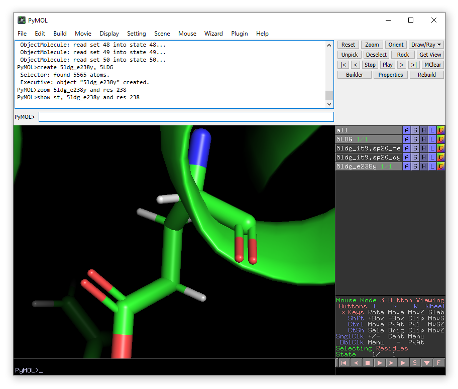
We will start by copying our object 5LDG to the new object 5ldg_e238y.

create 5ldg_e238y, 5LDG

We want to mutate Glu238 to Tyr, so we will show this residue in sticks and zoom in on it.

show st, 5ldg_e238y and res 238

zoom 5ldg_e238y and res 238

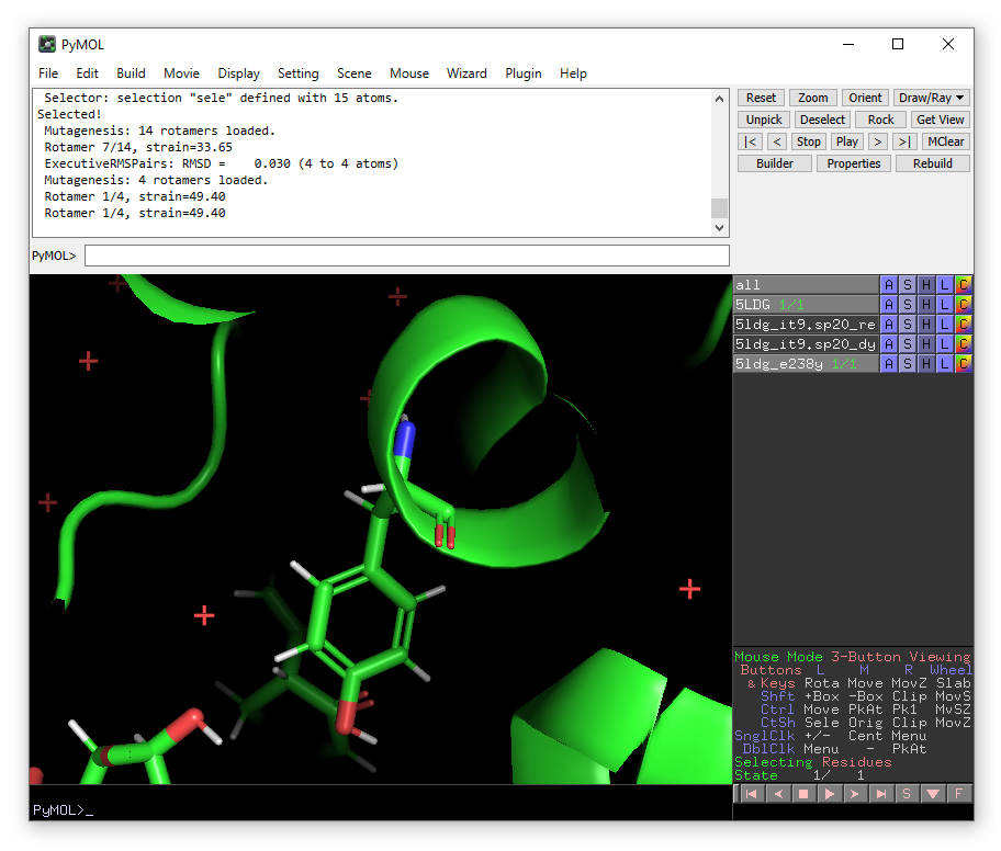
From the Wizard drop-down menu, select Mutagenesis -> Protein:

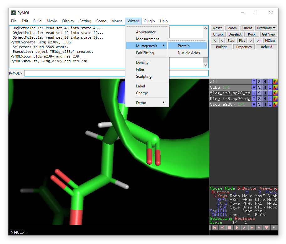
Click on Glu238 and then choose Tyr from the mutate to menu in the right-hand panel.

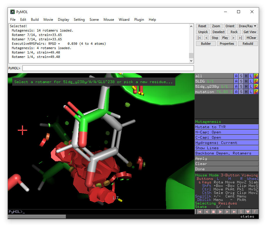
The lowest energy rotamer will then be displayed.

Even though in this case, there is a significant clash with the substrate IT9, go ahead and click apply to accept the mutation and then done to exit the wizard.

From the plugin menu choose Enlighten again.

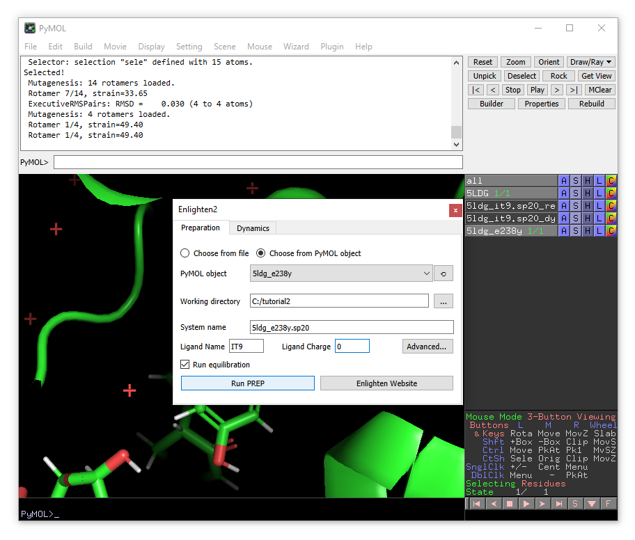
A new enlighten control panel will appear. To run simulations on the mutant model, ensure that the new 5ldg_e238y object is selected in the list and fill in the other fields similar to before (e.g. using 5ldg_e238y.sp20 as the system name). When done, click Run PREP (with Run equilibration ticked).

Once PREP is done, you will see that the object 5ldg_e238y.sp20_relax has been loaded. Note that there will be ‘bonds’ shown between the clashing Tyr238 and the substrate. You can remove the ‘bonds’ visualisation of the non-physical bonds using:

unbond resname IT9, res 234

Now you can run dynamics on the mutant model through Dynamics tab.

Part 4: Analysis

The MD trajectory should be automatically loaded into the objects when DYNAM is finished. Press the play button to move between the frames. You can adjust the number of frames per second in the Movie drop-down menu. You can use the measurement function in the Wizard menu to monitor distances during the MD simulation.

Zoom in on isopiperitenone (zoom resname IT9) and compare the position between wild-type (5LDG) and the E238Y mutant (5ldg_e238y). Also compare the position of the (mutated) residue, Glu238 or Tyr238 (both now renumbered as 234). You could now compare this to the proposed mechanisms in Scheme 2 of the paper, and see if the simulations can help you to explain the difference between wild-type IPR and IPR E238Y.

(Note that we simulated NADP+, not NADPH, and simulations were performed with the isopiperitenone substrate only. You could further extend this study by using NADPH and re-running simulations with menthone instead of isopiperitenone.)

---

Bugs in the Enlighten plugin or scripts can be reported as an “Issue” through the github site.

If you have in-depth feedback or thoughts about Enlighten you would like to share, please get in touch.

Thank you!